class: center, middle, inverse, title-slide # Introduction to Bioinformatics ## <del>with algorithms</del> ### Lijia Yu @ NCCL in China ### 2019/05/15<br/>(updated: 2019-06-03) --- background-image: url(https://image.slidesharecdn.com/bis2016introtobioinformatics-160909094908/95/introduction-to-bioinformatics-26-638.jpg) --- background-image: url(http://acm.na.edu/img/bioInfoLab/bioinformatics_venn.png) background-size: 350px background-position: 50% 65% # What is Bioinformatics? ### Bioinformatics is the field of science in which <u>biology</u>, <u>computer science</u>, and <u>information technology</u> merge into a single discipline. ¹ .footnote[ [1] Molecular Biology Review - NCBI [2] Venn diagram: http://acm.na.edu/img/bioInfoLab/bioinformatics_venn.png ] ??? The ultimate goal of the field is to enable the discovery of new biological insights as well as to create a global perspective from which unifying principles in biology can be discerned. - the development of new algorithms and statistics with which to assess relationships among members of large data sets - the analysis and interpretation of various types of data including nucleotide and amino acid sequences, protein domains, and protein structures - the development and implementation of tools that enable efficient access and management of different types of information --- <!-- # Milestones --> <!-- - In 1956, Symposium on Information Theory in Biology (Gatlinburg, USA). --> <!-- -- --> <!-- - In 1962, Zuckerkandl and Pauling's Molecular Clock --> <!--   --> <!-- ??? --> <!-- 在20世纪50年代前后，已有一些实验室开始测定蛋白质序列的信息，例如1947年测出短杆菌的五肽结构，1951年重构胰岛素的30个氨基酸，几乎在同一时期，科学家认识到DNA是遗传物质。 --> <!-- --- --> # 1. Molecular data collection and management - In 1979, <u>**GenBank**</u> was established at Los Alamos National Laboratory (USA). 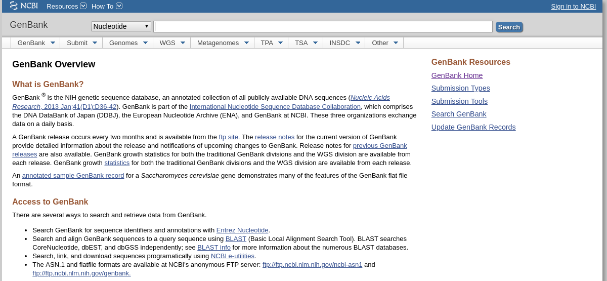 --- # 1. Molecular data collection and management - In 1979, <u>**GenBank**</u> was established at Los Alamos National Laboratory (USA). .center[] --- # 1. Molecular data collection and management - In 1982, nucleotide sequence database of European Molecular Biology Laboratory (also known as <u>**EMBL-Bank**</u>) was created (Europe).  ??? The EMBL Nucleotide Sequence Database (also known as EMBL-Bank) is the section of the ENA which contains high-level genome assembly details, as well as assembled sequences and their functional annotation. As of release 114 (December 2012), the EMBL Nucleotide Sequence Database contains approximately 5×1011 nucleotides with an uncompressed filesize of 1.6 terabytes. --- # 1. Molecular data collection and management - In 1986, DNA Data Bank of Japan (<u>**DDBJ**</u>) began data bank activities at National Institute of Genetics (Japan).  --- # 1. Molecular data collection and management - In the early 1990s, International Nucleotide Sequence Database Collaboration (INSDC) was founded in cooperation of Genebank/EMBL/DDBJ. .center[<img src="./2019-05-15-Introduction_to_Bioinformatics_files/figure/insdc.png" width="600">] --- # 1. Molecular data collection and management - Big Data Center: The Genome Sequence Archive (GSA) is a data repository for archiving raw sequence reads. .center[<img src="./2019-05-15-Introduction_to_Bioinformatics_files/figure/BIGD.png" width="600">] <!-- --- --> <!-- # 1. Molecular data collection and management --> <!-- ## Omics --> <!-- - Genomics --> <!-- - Comparative genomics --> <!-- - Functional genomics --> <!-- - Metagenomics --> <!-- - Neurogenomics --> <!-- - Pan-genomics --> <!-- - **Personal genomics** --> <!-- - Transcriptomics --> <!-- - Epigenomics --> <!-- - Proteomics --> --- # 2. Sequence alignment - In 1962, Zuckerkandl and Pauling introducing the concept of the "molecular clock", which enabled the neutral theory of molecular evolution. .center[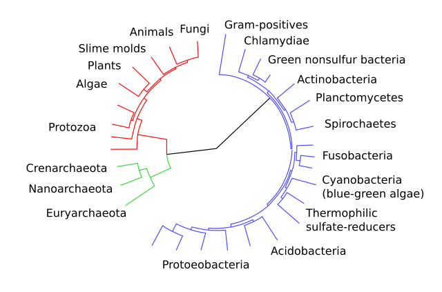] ??? In bioinformatics, a sequence alignment is a way of arranging the sequences of DNA, RNA, or protein to identify regions of similarity that may be a consequence of functional, structural, or evolutionary relationships between the sequences. 1962年莱纳斯·鲍林和艾美·祖柯坎（Emile Zuckerkandl）提出了分子时钟，透过比较同源蛋白质的差异来推算双方分歧的时间。 <!-- # 2. Sequence alignment --> <!-- .center[<img width="600" alt="Homology" src="http://image.slidesharecdn.com/ncbislides-110328185532-phpapp02/95/ncbi-boot-camp-for-beginners-slides-58-728.jpg">] --> --- # 2. Sequence alignment | position | 1 | 2 | 3 | 4 | 5 | 6 | 7 | 8 | 9 | 10 | 11 | 12 | 13 | 14 | |------------|---|---|---|---|---|---|---|---|---|---|---|---|---|---| | sequence 1 | G | C | A | T | G | A | C | G | A | A | T | C | A | G | | sequence 2 | T | A | T | G | A | C | A | A | A | C | A | G | C | | -- Delete(1,-) | position | 1 | 2 | 3 | 4 | 5 | 6 | 7 | 8 | 9 | 10 | 11 | 12 | 13 | 14 | |------------|---|---|---|---|---|---|---|---|---|---|---|---|---|---| | sequence 1 | G | C |<font color="red"> A </font> |<font color="red"> T </font> |<font color="red"> G </font>| <font color="red">A </font> | <font color="red">C </font>| G | <font color="red">A </font>|<font color="red"> A </font>| T | C | A | G | | sequence 2 | | T | <font color="red"> A </font>| <font color="red"> T </font> |<font color="red"> G </font>| <font color="red">A </font> | <font color="red">C </font>| A | <font color="red">A </font>|<font color="red"> A </font>| C | A | G | C | -- Delete(8,-) | position | 1 | 2 | 3 | 4 | 5 | 6 | 7 | 8 | 9 | 10 | 11 | 12 | 13 | 14 | 15 | |------------|---|---|---|---|---|---|---|---|---|---|---|---|---|---|---| | sequence 1 | G | C |<font color="red"> A </font> |<font color="red"> T </font> |<font color="red"> G </font>| <font color="red">A </font> | <font color="red">C </font>| G | <font color="red">A </font>|<font color="red"> A </font>| T | <font color="red">C </font>| <font color="red"> A </font>| <font color="red"> G </font> | | | sequence 2 | | T | <font color="red"> A </font>| <font color="red"> T </font> |<font color="red"> G </font>| <font color="red">A </font> | <font color="red">C </font>| -- |<font color="red">A </font>|<font color="red"> A </font>| A | <font color="red">C </font>| <font color="red"> A </font>| <font color="red"> G </font> | C | --- # 2. Sequence alignment - Hamming Distance -- | Hamming Distance(s,t)= | 2 | 3 | 5 | |:----------------------:|:---:|:-----:|:--------:| | s= | <font color="red"> A </font>A<font color="red"> T </font> | A<font color="red">GCA</font>A | A<font color="red"> GCAC</font>A<font color="red"> C</font>A | | t= | <font color="red"> T </font>A<font color="red"> A </font> | A<font color="red"> CAT</font>A | A<font color="red"> CACA</font>A<font color="red"> T</font>A | -- - scoring matrix |BLOSUM 62 Matrix|PAM 250 Matrix| |---|---| ||<img width="256" alt="PAM250" src="https://upload.wikimedia.org/wikipedia/commons/5/57/PAM250.png">| <!-- s=c("A","T","A") --> <!-- t=c("T","A","A") --> <!-- sum(s!=t) --> ??? BLOSUM矩阵由Henikoff提出，蛋白质短序列比对推导 PAM矩阵由Dayhoff提出，蛋白质全局序列比对推导 --- # 3. Genome Analysis | Genome | Where | Year | |--------------------------------------------------------------------|--------------------------|------| | H. Influenza | TIGR | 1995 | | E. Coli K-12 | Wisconsin | 1997 | | S. cerevisiae (yeast) | internat. collab. | 1997 | | C. elegans (worm) | Washington U./Sanger | 1998 | | Drosophila M. (fruit fly) | multiple groups | 2000 | | E. Coli 0157:H7 (pathogen) | Wisconsin | 2000 | | **H. Sapiens (that’s us)** | internat. collab./Celera | 2001 | | Mus musculus (mouse) | internat. collaboration | 2002 | | Oryza sativa L. ssp. indica & Oryza sativa L. ssp. japonica (rice) | internat. collaboration | 2002 | --- # 3. Genome Analysis - Cancer genome mutation .center[ <img width="600" alt="Driver_mutation" src="https://science.sciencemag.org/content/sci/339/6127/1546/F5.large.jpg">] .footnote[ [1] Cancer Genome Landscapes ] --- # 3. Genome Analysis - Genetic disease .center[ <img width="450" alt="gene_mutation_that_cause_huntington_disease" src="https://ghr.nlm.nih.gov/art/large/gene-mutation-that-causes-huntington-disease.jpeg">] .footnote[ [1] https://ghr.nlm.nih.gov/condition/huntington-disease#genes ] ??? The HTT mutation that causes Huntington disease involves a DNA segment known as a CAG trinucleotide repeat. --- <!-- # 4. Transcriptome Analysis --> <!-- - DNA microarry --> <!-- The original nucleic acid arrays were macro arrays approximately 9 cm × 12 cm and the first computerized image based analysis was published in 1981. It was invented by Patrick O. Brown. --> <!-- .center[] --> <!-- --- --> # 4. Transcriptome Analysis .center[] --- # 4. Transcriptome Analysis .center[] --- # 4. Transcriptome Analysis .center[<img width="350" alt="GeneExpressionHeatmap" src="https://upload.wikimedia.org/wikipedia/commons/thumb/4/48/Heatmap.png/480px-Heatmap.png"><img width="350" alt="GeneNetwork" src="https://upload.wikimedia.org/wikipedia/en/thumb/8/8e/ExampleNet.png/488px-ExampleNet.png">] --- # 5. Proteome Analysis  .footnote[ [1] https://ib.bioninja.com.au/standard-level/topic-2-molecular-biology/24-proteins/proteome.html ] --- # 5. Proteome Analysis .center[] .footnote[ [1] [Introduction to Practical Biochemistry ](https://www.tankonyvtar.hu/en/tartalom/tamop412A/2011-0073_introduction_practical_biochemistry/ch11s03.html) <!-- (http://elte.prompt.hu/sites/default/files/tananyagok/IntroductionToPracticalBiochemistry/ch11s03.html) --> ] --- # 5. Proteome Analysis .center[] --- # Related knowledge 1. Biology: **Cell Biology**, **Molecular Biology**, Biochemistry, Developmental Biology, **Genomics**, **Genetics**, etc. -- 2. Programming: **R**, Perl/**Python**, C/C++, etc. -- 3. Statistics: **Hypothesis test**, **Interval estimation**, **Significance**, **Regression**, etc. <!--.center[]--> --- # Bioinformatics in Action - High performance computing .center[] .footnote[ [1] [Multiple users concept](http://help.mamut.com/uk/mhelp/rtm/administrator/installation/server/multi_user_concept.htm) ] --- background-image: url(https://upload.wikimedia.org/wikipedia/commons/thumb/1/1b/R_logo.svg/310px-R_logo.svg.png) background-size: 100px background-position: 90% 8% .left-column[ ## What is R? ] .right-column[ <br/> <br/> <br/> <br/> **R** is a language and environment for statistical computing and graphics. Designed by: **R**oss Ihaka, **R**obert Gentleman. ```r x <- 1:6 # Create vector. y <- x^2 # Create vector by formula. plot(x,y,type = "b") ``` <!-- --> ] --- .left-column[ ## What is R? ## What is RStudio? ] .right-column[   ] --- # RStudio Server with Terminal  -- - Login to 192.168.0.105:8787 --- # Syllabus - Basic knowledge of Linux - NGS Data analysis (Genome data) - NGS analysis online tools and Database # Resource [1] [Bioinformatics (For undergraduates)](http://xue.biocuckoo.org/course.html) (in Chinese) .footnote[ * All pictures without footnote are getting from Wikipedia or browser snapshots. ] --- class: center, middle # Thanks! Slides created via the R package [**xaringan**](https://github.com/yihui/xaringan). The chakra comes from [remark.js](https://remarkjs.com), [**knitr**](http://yihui.name/knitr), and [R Markdown](https://rmarkdown.rstudio.com).